Page 22 - PA_Enterprise_January-2025

PAE

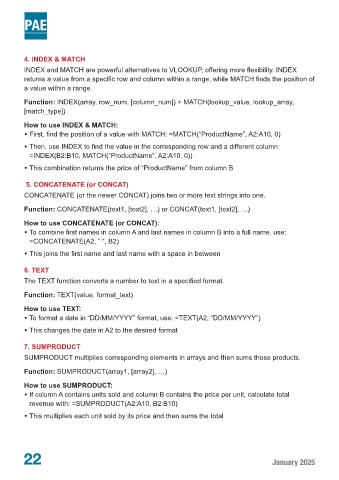
4. INDEX & MATCH
INDEX and MATCH are powerful alternatives to VLOOKUP, offering more flexibility. INDEX
returns a value from a specific row and column within a range, while MATCH finds the position of
a value within a range.

Function: INDEX(array, row_num, [column_num]) + MATCH(lookup_value, lookup_array,
[match_type])

How to use INDEX & MATCH:
• First, find the position of a value with MATCH: =MATCH(“ProductName”, A2:A10, 0)

• Then, use INDEX to find the value in the corresponding row and a different column:
=INDEX(B2:B10, MATCH(“ProductName”, A2:A10, 0))

• This combination returns the price of “ProductName” from column B

5. CONCATENATE (or CONCAT)

CONCATENATE (or the newer CONCAT) joins two or more text strings into one.

Function: CONCATENATE(text1, [text2], …) or CONCAT(text1, [text2], …)

How to use CONCATENATE (or CONCAT):
• To combine first names in column A and last names in column B into a full name, use:
=CONCATENATE(A2, ” “, B2)

• This joins the first name and last name with a space in between

6. TEXT

The TEXT function converts a number to text in a specified format.

Function: TEXT(value, format_text)

How to use TEXT:
• To format a date in “DD/MM/YYYY” format, use: =TEXT(A2, “DD/MM/YYYY”)
• This changes the date in A2 to the desired format

7. SUMPRODUCT
SUMPRODUCT multiplies corresponding elements in arrays and then sums those products.

Function: SUMPRODUCT(array1, [array2], …)

How to use SUMPRODUCT:
• If column A contains units sold and column B contains the price per unit, calculate total
revenue with: =SUMPRODUCT(A2:A10, B2:B10)
• This multiplies each unit sold by its price and then sums the total

22 January 2025